Gradient descent is the most popular optimization technique in machine learning (ML) modeling. The algorithm minimizes the error between the predicted values and the ground truth. Since the technique considers each data point to understand and minimize the error, its performance depends on the training data size. Techniques like Stochastic Gradient Descent (SGD) are designed to improve the calculation performance but at the cost of convergence accuracy.
Stochastic Average Gradient balances the classic approach, known as Full Gradient Descent and SGD, and offers both benefits. But before we can use the algorithm, we must first understand its significance for model optimization.
Optimizing Machine Learning Objectives with Gradient Descent
Every ML algorithm has an associated loss function that aims to minimize or improve the model’s performance. Mathematically, the loss can be defined as:
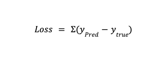
It is simply the difference between the actual and the predicted output, and minimizing this difference means that our model comes closer to the ground truth values.
The minimization algorithm uses gradient descent to traverse the loss function and find a global minimum. Each traversal step involves updating the algorithm's weights to optimize the output.
Plain Gradient Descent
The conventional gradient descent algorithm uses the average of all the gradients calculated across the entire dataset. The lifecycle of a single training example looks like the following:

The weight update equation looks like the following:
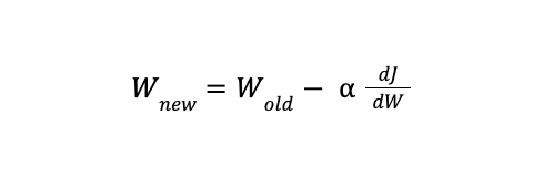
Where W represents the model weights and dJ/dW is the derivative of the loss function with respect to the model weight. The conventional method has a high convergence rate but becomes computationally expensive when dealing with large datasets comprising millions of data points.
Stochastic Gradient Descent (SGD)
The SGD methodology remains the same as plain GD, but instead of using the entire dataset to calculate the gradients, it uses a small batch from the inputs. The method is much more efficient but may hop too much around the global minima since each iteration uses only a part of the data for learning.
Stochastic Average Gradient
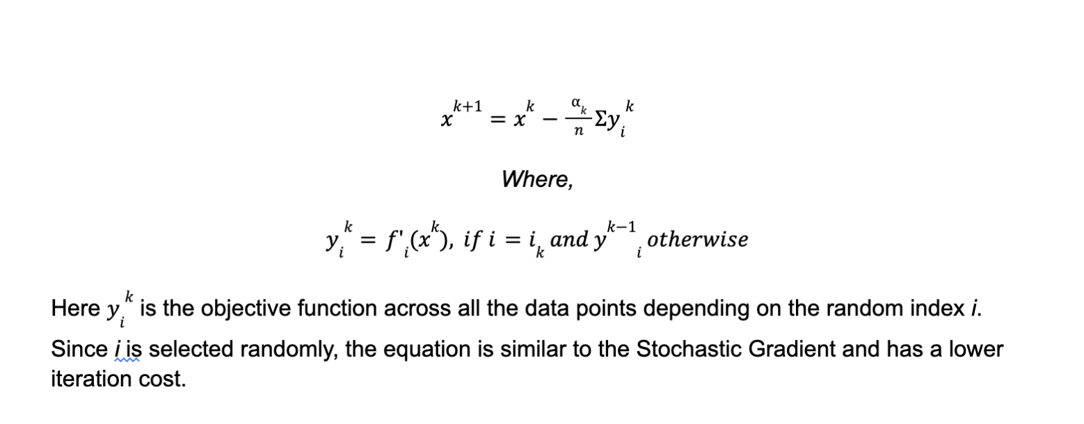
The Stochastic Average Gradient (SAG) approach was introduced as a middle ground between GD and SGD. It selects a random data point and updates its value based on the gradient at that point and a weighted average of the past gradients stored for that particular data point.
Similar to SGD, SAG models every problem as a finite sum of convex, differentiable functions. At any given iteration, it uses the present gradients and the average of previous gradients for weight updation. The equation takes the following form:
Convergence Rate
Between the two popular algorithms, full gradient (FG) and stochastic gradient descent (SGD), the FG algorithm has a better convergence rate since it utilizes the entire data set during each iteration for calculation.
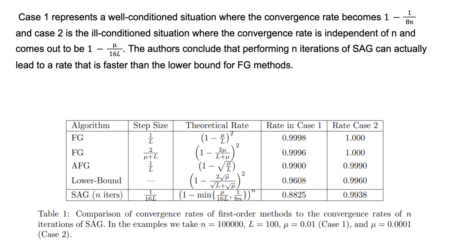
Although SAG has a structure similar to SGD, its convergence rate is comparable to and sometimes better than the full gradient approach. Table 1 below summarizes the results from the experiments of
Further Modifications
Despite its amazing performance, several modifications have been proposed to the original SGD algorithm to help improve performance.
- Re-weighting in Early Iterations: SAG convergence remains slow during the first few iterations since the algorithm normalizes the direction with n (total number of data points). This provides an inaccurate estimate as the algorithm has yet to see many data points. The modification suggests normalizing by the m instead of n, where m is the number of data points seen at least once until that particular iteration.
- Mini-batches: The Stochastic Gradient approach uses mini-batches to process multiple data points simultaneously. The same approach can be applied to SAG. This allows for vectorization and parallelization for improved computer efficiency. It also reduces memory load, a prominent challenge for the SAG algorithm.
- Step-Size experimentation: The step size mentioned earlier (116L) provides amazing results, but the authors further experimented by using the step size of 1L. The latter provided even better convergence. However, the authors were unable to present a formal analysis of the improved results. They conclude that the step size should be experimented with to find the optimal one for the specific problem.
Final Thoughts
Gradient descent is a popular optimization used for locating global minima of the provided objective functions. The algorithm uses the gradient of the objective function to traverse the function slope until it reaches the lowest point.
Full Gradient Descent (FG) and Stochastic Gradient Descent (SGD) are two popular variations of the algorithm. FG uses the entire dataset during each iteration and provides a high convergence rate at a high computation cost. At each iteration, SGD uses a subset of data to run the algorithm. It is far more efficient but with an uncertain convergence.
Stochastic Average Gradient (SAG) is another variation that provides the benefits of both previous algorithms. It uses the average of past gradients and a subset of the dataset to provide a high convergence rate with low computation. The algorithm can be further modified to improve its efficiency using vectorization and mini-batches.