Revealing Gender Bias: Insights from Blind Auditions on 'The Voice

Table of Links

Abstract

Background

Data

Methodology

Results

Discussion and Conclusion, and References

A Appendix Tables and Figures

2 Data

I used the blind audition part of the show as a natural experiment in this work. The data on a blind audition was compiled from historical Voice TV shows on Wikipedia. I web-scraped the results of the blind audition for four countries: the UK, France, Germany, and Australia. Each country held approximately ten seasons each year, starting from the year 2012. Each country’s Voice Wiki page is divided by season, each season is divided by the episodes, and the order of the performance splits each episode. The page includes the singer and coach’s information, the singer’s age, the order of performance, and the song.

From the Wiki page, I constructed the outcome variable based on the coaches who pressed the button if the coach chose the specific artist. Thus, I can build the result of the four coaches for each artist. Similarly, the page provides the actual order of the performance. Since the primary goal of the analysis is to identify gender-specific preferences, I needed to determine the gender of the artist.

I infer the gender of the artists based on their first names. I used an online application programming interface (API) called Genderize.io. The application has pre-trained machine learning algorithms that are used to predict gender. The API gives a confidence level in probabilistic terms and the exact name count in their already used datasets. Utilizing a threshold of 90% probability, I am able to attach a gender to approximately 97% of the whole dataset. For the remaining 3% of the first names, I hardcoded by checking the performance on the YouTube webpage. The gender of the coaches can easily be identified as all of them are well-established artists.

I also used the genre of the song the artist performs. Using song information from the Wikipedia page, I extracted the genre of the music from the Spotify API. The API gives multiple genres that correspond to the given song. By doing frequency distribution, I determined the most frequent genres and came up with the eleven unique genres.

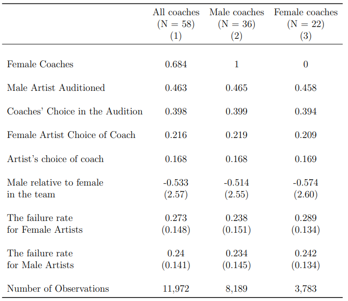
Summary statistics are shown at the coach level in Table 1. Column (1) includes all coaches in the sample, while Columns (2) and (3) disaggregate to coaches who are female or male, respectively. The data has 11,972 observations, 58 unique coaches, and 3,009 unique artists. 31.6 percent of the coaches were female, though there is considerable heterogeneity across the team gender composition and failure rates for female and male artists. Similarly, about 46.3 percent of artists are men, providing decent statistical power for an own-gender bias analysis.

My primary analysis includes all the coaches’ choices, with approximately 40 percent of the artists being chosen in the blind audition round. Female artists are chosen about 21.6 percent of the time. The difference between female coaches and male coaches choosing female artists is a 1 percent difference. This pattern of having a 1% difference continues to hold for the male artists who are chosen 18 percent of the time. Thus, a naive comparison of the raw data for female and male gender would yield a conclusion of no gender bias. Since the preference of female and male artists across female and male coaches is similar, the selection difference lies at about one percent. To justify this premise, I examine the order of each performance at the artist level and how TV show-related specification affects decision-making.

Table 1 also provides summary statistics for TV show-related specifications, considering them heterogeneous in the analysis. Each coach and artist has a unique specification, such as the order of their performance, their preference towards a specific coach, and the genre of the song. Ultimately, 16.8 percent of the artists ended up on a team. From that team configuration, we can determine the gender composition of the team, which is the number of women and men on the team during the blind audition stage. The average difference between the number of males and females for each order on the team is -0.533, meaning that the number of female artists is 0.5 people higher on average compared with the male artists. Additional information is obtained when two or more coaches pursue the same artist, providing the artist with the final choice. I estimated the failure rate for these cases, and each coach has about a 0.27 failure rate for female artists and 0.24 for male artists. This is the rate at which a coach wanted an artist of a particular gender on their team, and the artist did not choose the coach. Both of these variables have considerable differences across the gender of the coach, which enriches our study to identify own-gender bias in the selection process.

Notes: This table presents summary statistics for the estimation sample. The unit of observation is performance in the blind audition stage. The table shows statistics of all performances for which artists and drivers are men and women. The sample includes four countries, and each country has ten seasons. Standard deviations in parentheses. All values reported in this table are unconditional average rates of the variables indicated in rows.

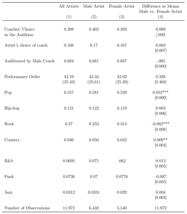
As discussed and shown in the Section 1, the institutional setting provides for the exogenous assignment of gender encounters between coach and artist. Table 2 examines this exogeneity assumption by estimating differences in the observed characteristics of male and female artists. The first column shows mean characteristics for all artists, while the second and third columns present average outcomes for male and female artists. The fourth column reports the difference between the two means. Comparing overall raw means is consistent with the assignment procedure described above. There is no significant difference between male and female artists in any show-related specifications, such as being chosen by coaches, selecting a team, being chosen by a male coach, and the order of their performance. This supports our identification strategy: in a given show setting, there is little evidence to suggest that male artists’ performances systematically differ from those performed by female ones. However, I also find some statistically significant differences. For example, male artists are 5.2 percent more likely to perform pop genre songs. Similarly, the share of classic style and the share of rock style is lower, while the share of country style is higher among male artists. All these significant observables will be estimated in the setting as confounding factors.

Notes: Standard deviations in parentheses in columns 1,2 and 3. Each entry in column 4 is derived from a separate OLS regression where explanatory variable is indicator for male artist. * p < 0.1, ** p < 0.05, *** p < 0.01