Colliding Magnetospheres in The Young High-Eccentricity Binary DQ Tau: Flare Analyses

Table of Links

• Abstract and Intro
• X-ray Observations and Data Extraction
• Flare Analyses
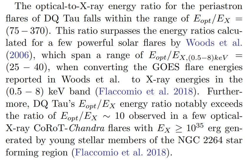
• Comparison with X-ray Flares from Young Stars
• Discussion
• Conclusions
• Acknowledgments and References

3. FLARE ANALYSES

3.1. Detection of Flares

Figures 2a,b and 3a,b display the X-ray lightcurves and temporal evolution of the median energy for the X-ray events detected within the circular extraction regions depicted in Figure 1.

In the shown lightcurve and median energy plots for NuSTAR, individual data points represent bins containing 30 X-ray events from the combined FPMA and FPMB data. Conversely, each point in the Swift-XRT and Chandra lightcurves and median energy plots corresponds to a single X-ray observation.

The X-ray lightcurve from NuSTAR provides clear evidence of the occurrence of at least two X-ray flaring events within the orbital phase range of (0.96−1.1). The first (main) flare is identified by solid red curves representing exponential fits to the rise and decay phases, while the second flare is indicated by the decay data fit. These fits were performed using the observed binned count rate data, as described in equation (B1) and detailed in Getman et al. (2021). The resulting time scales are as follows: an 80 ± 19 ksec rise time (τrise) for the main flare and decay times (τdecay) of 49 ± 12 ksec and 52±13 ksec for the main and second flares, respectively. Such decay time scales are commonly observed in large X-ray flares detected in numerous young stellar members of various nearby star-forming regions (Getman et al. 2008; Getman & Feigelson 2021). However, the main flare’s long rise time is longer than that of typical large X-ray flares, reminiscent of rare slow-rise-top-flat flares observed in a dozen young stellar members of the Orion Nebula Cluster (Getman et al. 2008).

The approximate observed peak level of the main Xray flare is indicated by the upper dashed line in Figure 2. It surpasses the ”characteristic” level (baseline) of X-ray emission (Wolk et al. 2005; Caramazza et al. 2007), represented by the lower dashed line, by a factor of 3. The characteristic level likely corresponds to the combined effect of numerous unresolved micro-flares and nano-flares. The decay time-scale and amplitude of the main flare bear resemblance to those measured for the large X-ray flares captured near DQ Tau’s periastron by Chandra and Swift-XRT in 2010 and 2021 (Getman et al. 2011, 2022a).

The Swift-XRT data, despite lower cadence and counting statistics, exhibit a similar morphology to the NuSTAR DQ Tau flares. Moreover, both the X-ray median energies from NuSTAR and Swift-XRT display temporal evolution patterns of rise and decay within the orbital phase range of (0.96 − 1.1). The median energy serves as a proxy for plasma temperature, and these temperature evolutionary patterns are characteristic of X-ray flares fueled by magnetic reconnection processes (Getman et al. 2008, 2011, 2021).

Furthermore, the NuSTAR and Swift-XRT light curves suggest the presence of additional X-ray flaring events occurring beyond the orbital phase of 1.1. We postulate the existence of at least two significant X-ray flares within the orbital phase intervals of (1.1 − 1.17) and (1.17 − 1.21). These events are designated as the third and fourth X-ray flares, respectively. The third flare may comprise smaller flares within it. Our estimates for the rise and decay timescales of the third flare, derived from a combination of NuSTAR and Swift-XRT data points, are τrise = 40±10 ks and τdecay = 33±11 ks, as indicated by the grey dashed lines in Figure 2a. These measurements are only approximate due to differences between the NuSTAR and Swift-XRT data points near orbital phases 1.11 and 1.13, which may suggest a more complex flare morphology. Unfortunately, we lack sufficient Swift-XRT data to determine the timescales for the fourth flare.

Figures 2c,d illustrate the Swift-UVOT lightcurves for the six UVOT filters. While the longer time-scale UVOT variation may be linked to the known increased accretion rate of material from the circumbinary disk onto both stellar components during periastron passages (Fiorellino et al. 2022, and references therein), the shorter time-scale variation, occurring within the (0.96 − 1.1) orbital phase range, is associated with the main and second X-ray flares. The classical non-thermal thick-target model, frequently applied to solar and stellar flares (Brown 1971; Lin & Hudson 1976), predicts an optical component to accompany an X-ray flare. The simultaneous appearance of the Swift-UVOT and NuSTAR+Swift-XRT brightening events is qualitatively in line with the model predictions and suggests that both X-ray and UVOT emissions trace the same astrophysical phenomenon. It also aligns with empirical data on optical-X-ray flares observed in young members of the NGC 2264 star-forming region (Flaccomio et al. 2018).

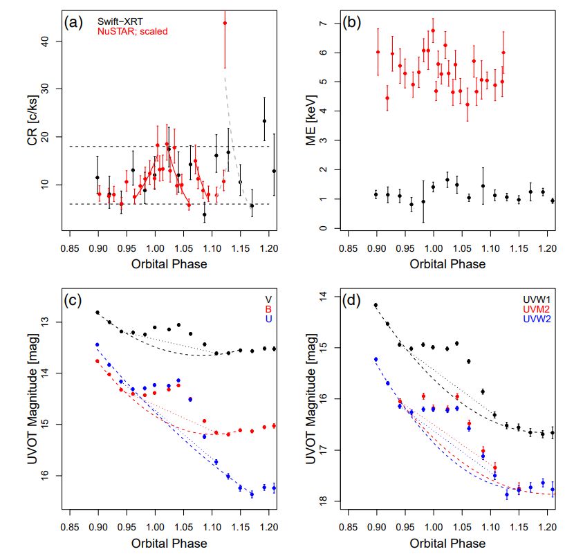
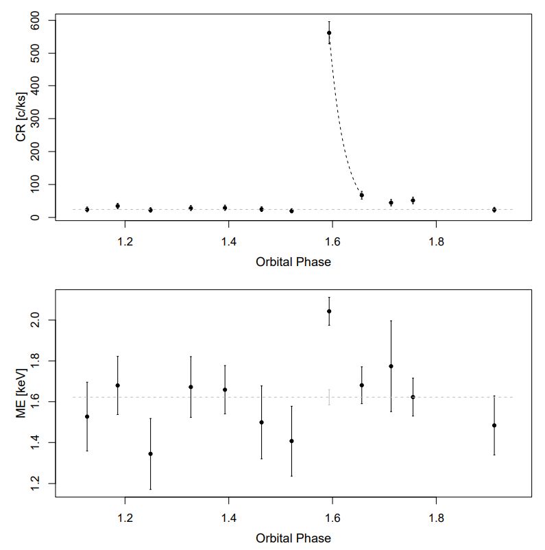
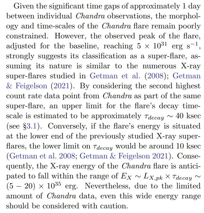
Figure 3 showcases our Chandra observation made at orbital phases away from the periastron, capturing a potent X-ray flare. The observed peak count rate (ObsID 26471; orbital phase 1.60), uncorrected for pileup effects, exceeds the characteristic count rate level (represented by the grey dashed line) by a factor greater than 20. If the Chandra data point with the second highest count rate (ObsID 26472; orbital phase 1.66) is linked to the same flare, then the exponential decay time scale (marked by the black dashed line) may extend up to 40 ksec. Notably, the X-ray median energy at the observed peak of the flare, as measured from the ObsID 24671 data, significantly surpasses the values obtained from the combined data of the other 11 Chandra observations (illustrated by the grey dashed line with the accompanying grey solid error bar), indicating a hotter plasma state during the flare. The conclusive evidence for this finding will be provided by the Chandra pileupcorrected spectroscopy, which will be discussed in detail in §3.2.

3.2. Spectral Analyses Of Flares and Characteristic Emission

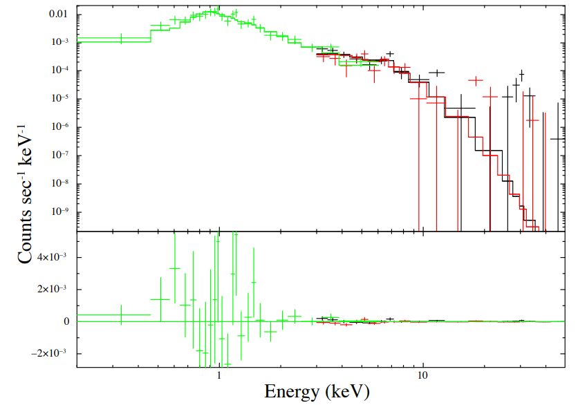
The NuSTAR and Swift-XRT data cover a similar orbital phase range, but they provide only modest counting statistics. Consequently, only basic spectral properties, such as the time-integrated hot plasma temperature component and X-ray luminosities (specifically for the characteristic and peak main flare states), can be reliably determined1 . To achieve this, we performed simultaneous fitting of the stacked Swift-XRT spectrum from the 16 observations and the individual NuSTAR FPMA and FPMB spectra. The Swift-XRT spectrum was binned to a minimum of 10 counts per bin, whereas the NuSTAR spectra were binned to 40 counts per bin. We employed the simple absorbed two-temperature optically thin thermal plasma model using the XSPEC package (Arnaud 1996) and employed Gehrels χ 2 statistics (Gehrels 1986) for the data fitting. The model used was tbabs × (apec + apec), where tbabs (Wilms et al. 2000) and apec (Smith et al. 2001) represent the absorption and plasma emission model components, respectively. Considering the low counting statistics, certain parameters were held fixed at characteristic values. Specifically, the coronal elemental abundances, the soft temperature component (kT1), and the column density (NH) were all set to their respective characteristic values. The coronal elemental abundances were fixed at 0.3 times solar elemental abundances (Imanishi et al. 2001; Feigelson et al. 2002, for young stars), the soft temperature component (kT1) was set to 0.8 keV (Preibisch et al. 2005; Getman et al. 2010, for young stars), and the column density (NH) was held at 1.3 × 1021cm−2 (Getman et al. 2011, for DQ Tau).

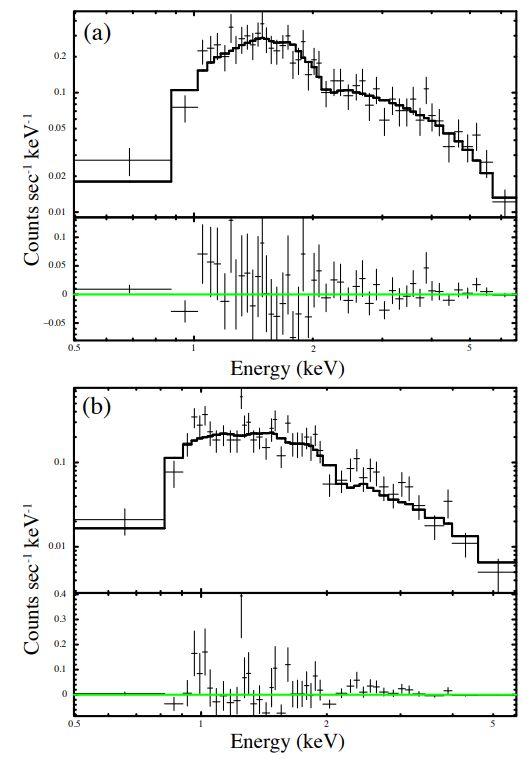
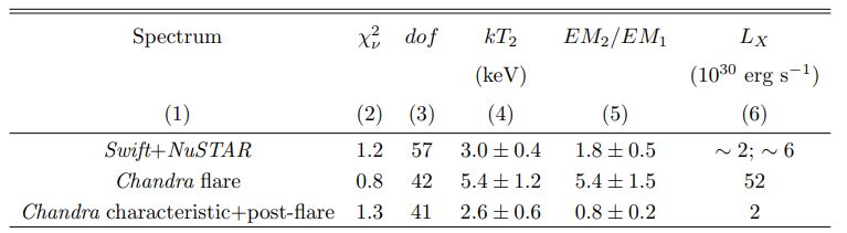
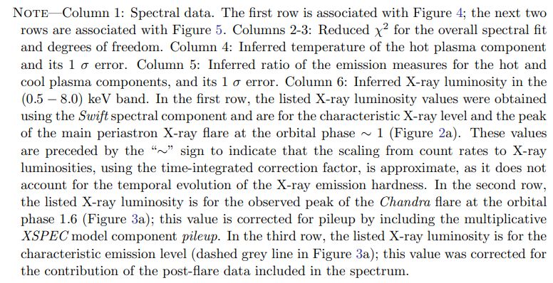
Figure 4 showcases the Swift-XRT and NuSTAR spectra along with the best-fit model obtained from the simultaneous fit. The corresponding spectral fitting results can be found in Table 1. To determine the X-ray luminosities, the count rate of the Swift-XRT spectrum was scaled to the count rate levels corresponding to the peak of the main flare and characteristic states shown in Figure 2 (dashed lines).

Furthermore, the inclusion of the powerlaw model component to search for non-thermal X-ray emission did not yield an improved fit, confirming the findings of Figure 1b, where it was evident that the NuSTAR data beyond 10 keV were predominantly influenced by the background.

In contrast to the Swift-XRT and NuSTAR data, the Chandra data provide a sufficient number of X-ray counts, allowing for the creation of two distinct spectra. One spectrum is derived from the data of a single observation (ObsID 26471) characterized by the highest count rate, representing the observed flare peak. The second spectrum is based on the data from the remaining 11 Chandra observations, corresponding to the characteristic and post-flare states. To ensure reliable analysis, the ”observed flare peak” and ”characteristic + post-flare” spectra were binned, with a minimum of 15 counts per bin for the former and 10 counts per bin for the latter.

The Chandra ”characteristic + post-flare” spectrum was fitted using the same model and fixed parameters employed for the NuSTAR and Swift-XRT spectra. However, for the flare peak spectrum, as the ObsID 26471 data are affected by pileup, the pileup model described by Davis (2001) was applied, along with tbabs×(apec+apec), to correct for this effect. Only the grade morphing α and PSF fraction psffrac parameters were varied within the pileup model. The best-fit parameters are α = 0.9 and psffrac = 0.98. The spectral fitting of Chandra data is illustrated in Figure 5, with the corresponding results summarized in Table 1.

3.3. Flare Energetics and Loop Length

3.3.1. X-ray Energy Of Periastron Flares

We have estimated the energy values of three X-ray flares occurring near periastron, referred to as the main, second, and third flares. This estimation involves integrating the count rates from NuSTAR and Swift-XRT, as shown in Figure 2a. These counts were corrected for the baseline and transformed into intrinsic X-ray luminosities, all within the duration of the respective flares. We excluded the outlier Swift-XRT point at orbital phase 1.11 from the calculation of the third flare’s energy, as it may be related to a smaller unresolved flare.

3.3.2. Optical and Near-Ultraviolet Energies Of Periastron Flares

Here, we categorize the Swift-UVOT observations into two groups: optical and near-ultraviolet (NUV). The optical data correspond to measurements taken with the V , B, and U filters, which have central wavelengths of 547 nm, 439 nm, and 346 nm, respectively. On the other hand, the NUV data correspond to observations made with the W1, M2, and W2 filters, which have central wavelengths of 260 nm, 225 nm, and 193 nm, respectively. Note that several Swift-UVOT observations lack data in the M2 filter (Figure 2), resulting in fewer NUV data points than optical points used in the analyses below.

Figure 2 illustrates that the main and second X-ray periastron flares detected by NuSTAR and Swift-XRT are accompanied by significant optical and NUV flares detected by Swift-UVOT.

Due to the limited number of data points in the UVOT observations (6 per individual orbital phase), our data fitting is restricted to a simple blackbody model. However, Brasseur et al. (2023) argue that such simplistic models may not adequately fit both the NUV and optical flare data simultaneously, considering the time- and wavelength-dependent optical depths of flare emission in the lower stellar atmosphere. We confirm their assertion by finding that fitting DQ Tau’s combined NUV and optical flare data with a one-temperature blackbody model yields a poor fit (not shown here). Therefore, our focus shifts towards fitting the NUV and optical components of the flares separately.

For the orbital range Φ = (0.96 − 1.1), a preliminary estimation is conducted to determine the combined energy of the main and secondary flares during periastron. Firstly, the V -, B-, and U-band UVOT fluxes are adjusted by subtracting two different baseline levels, as indicated by the dashed and dotted lines in Figure 2c. The start and end points of the optical/NUV flares are determined through visual inspection of the UVOT light curves in Figure 2. These points correspond to orbital phase instances with significant changes in the decay slopes of the UVOT light curves. The UVOT data outside the flares were used in the regression analysis to obtain baseline polynomial fits.

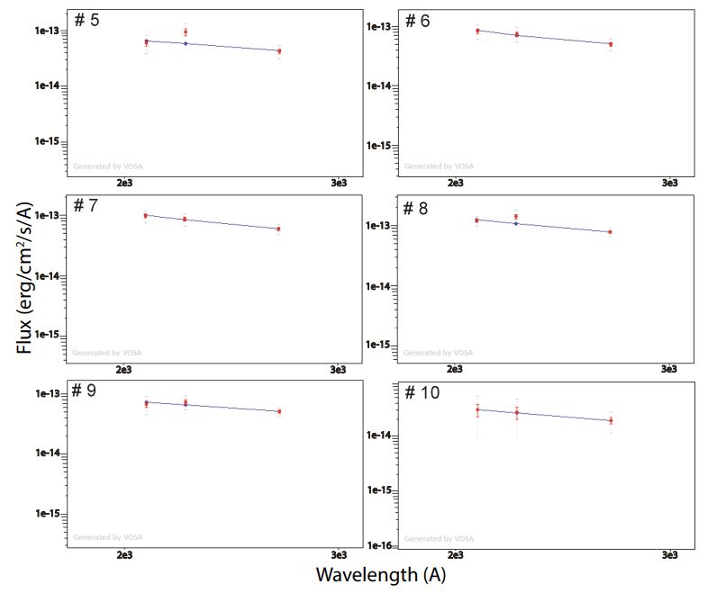
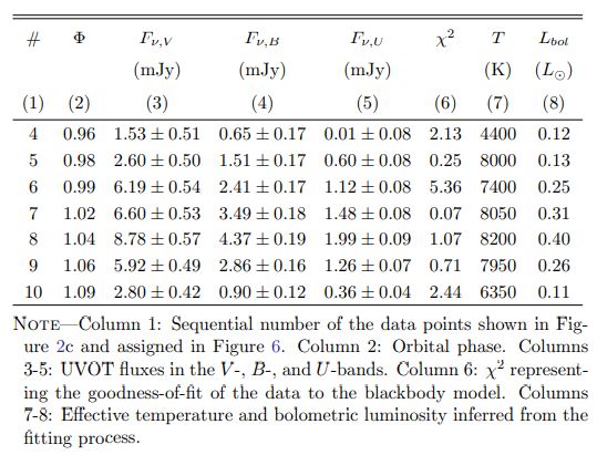
Subsequently, the VOSA SED (spectral energy distribution) analyzer (Bayo et al. 2008) is utilized to fit these two sets of flux data using the blackbody model (Figure 6). The visual source extinction is fixed at AV = 1.7 mag (Fiorellino et al. 2022). The effective temperature model parameter is constrained within a range of (4000 − 14000) K, which aligns with the temperatures observed in Solar and stellar flares (Kowalski et al. 2013; Flaccomio et al. 2018), as well as the temperatures found in accretion hot-spots (Tofflemire et al. 2017). The best-fit results for the version with the polynomial baseline are presented in Table 2 and Figure 6. For most data points, the inferred temperatures closely align with T ∼ 8000 K, consistent with the assumed temperatures of T = 9000 − 10000 K for the Sun and young NGC 2264 stars (Kretzschmar 2011; Flaccomio et al. 2018). For the version with the linear baseline, the inferred temperatures appear even closer to T ∼ 10000 K. However, it is important to note that such temperature values are also applicable to accretion hot spots on DQ Tau and other stars Tofflemire et al. (2017). The formal statistical errors on the inferred bolometric luminosities are less than 1%.

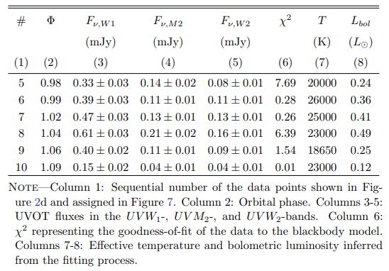
The fitting procedure for the NUV flare is performed similarly, with the initial blackbody temperature parameter upper boundary raised to 36000 K as considered for GALEX-NUV stellar flares in Brasseur et al. (2023). Such a range also includes the temperature value of 25000 K proposed for the UV component of solar “white-light” flares (Fletcher et al. 2007). The best-fit results for the version with the polynomial baseline are presented in Table 3 and Figure 7. The temperatures inferred for the DQ Tau flares fall within the range of (18000 − 26000) K, closely resembling the high blackbody temperatures typically associated with solar flares. However, it is worth noting that these elevated temperatures may also be attributed to the accreting material in the vicinity of the shock regions (Sicilia-Aguilar et al. 2015).

3.3.4. Flaring Coronal Loop Length Near Periastron

Within the framework of the time-dependent hydrodynamic model proposed by Reale et al. (1997); Reale (2007), a preliminary estimation of the coronal loop length can be made for the primary X-ray periastron flare. This model is applicable in cases where flaring multi-loop arcades are present, with the flare being predominantly governed by a single loop or multiple individual loop events that exhibit similar temperature and emission measure temporal profiles, occurring almost simultaneously (Reale 2014; Getman et al. 2011).